Data Exploration
Data Table
In this study, the experimental unit is each individual willow plant (1 plant per pot). The predictor (or dependent) variables are the capping depths (0cm, 5cm, 10cm, 20cm) and soil type/treatment (forest floor mineral mix, peat mineral mix, 50/50 mix, clay subsoil with 50/50mix topsoil, saline clay subsoil with 50/50 mix topsoil, biochar added to 50/50 mix topsoil). The predictor variables are manipulated to affect the response variables. The response (or independent) variables are height (cm), diameter (mm), and aboveground biomass (g). Soil type/treatment is a nominal, categorical variable. Capping depth is an ordinal, categorical variable. Finally, all response variables are continuous, ratio variables.
In this study, the experimental unit is each individual willow plant (1 plant per pot). The predictor (or dependent) variables are the capping depths (0cm, 5cm, 10cm, 20cm) and soil type/treatment (forest floor mineral mix, peat mineral mix, 50/50 mix, clay subsoil with 50/50mix topsoil, saline clay subsoil with 50/50 mix topsoil, biochar added to 50/50 mix topsoil). The predictor variables are manipulated to affect the response variables. The response (or independent) variables are height (cm), diameter (mm), and aboveground biomass (g). Soil type/treatment is a nominal, categorical variable. Capping depth is an ordinal, categorical variable. Finally, all response variables are continuous, ratio variables.
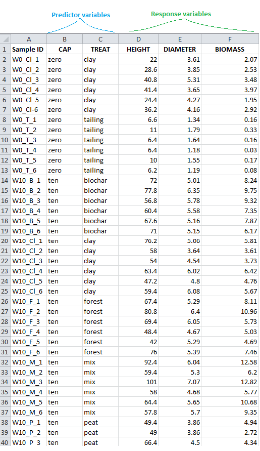
Figure 7. Simplified data table.
Exploratory Graphics
In order to determine what sort of sample distribution occurred in my results, I plotted histograms for each response variable (Figure 8). Although ‘biomass’ seems to resemble the closest to a normal distribution, all three response variable histograms have outliers. The ‘height’ histogram least of all resembles a normal distribution, while ‘stem diameter’ has a very nice distribution when ignoring the 1-2 mm outliers. These outliers are a result of the willow growth being severely impacted when grown directly in tailings material.
Considering the similarity in quality of the three response variables (as they are all growth responses), I wanted to verify if there was in fact a quantifiable similarity between the three. In order to visualize this, I plotted several scatter plots (Figure 9) that show the relationship between each variable through regression analysis. The data demonstrates a positive relationship between height, diameter and biomass. For this reason, as well as the distributions found in Figure 8, I will only focus on aboveground biomass when further analyzing the results.
To meet the ANOVA assumption of normal distribution, box plots were visualized for sub-experiments 1 and 2 (see Figure 10-a and 10-b).
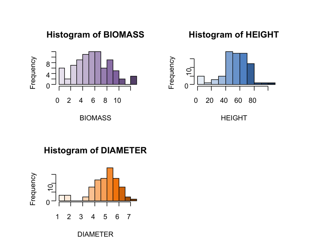
Figure 8. Histograms for biomass, height and diameter variables.
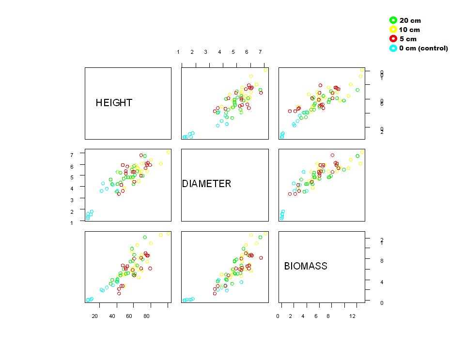
Figure 9. Scatter plots of height, diameter and biomass variables
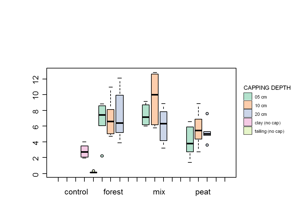
Figure 10-a. Boxplots of treatments and capping depths vs biomass for sub-experiment 1.
|
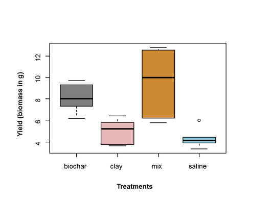
Figure 10-b. Boxplots of treatments vs biomass for sub-experiment 2.
|
Statistical Analysis
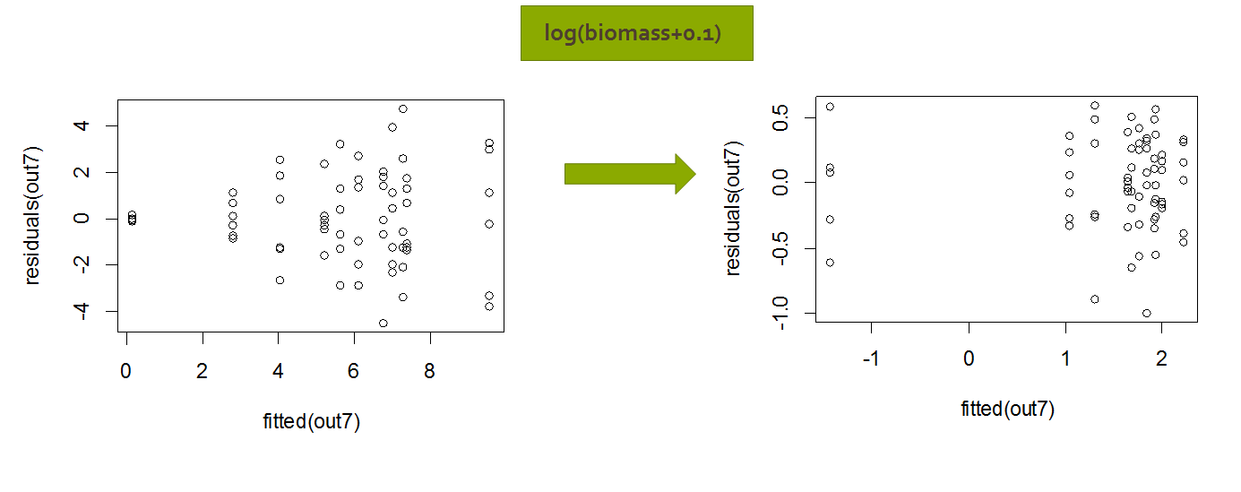
That data met the ANOVA assumptions of independence and normal distribution (see Figure 8, 10-a and 10-b). However, after plotting the residuals (plot(residuals~fitted), it was determined that the assumption of homogeneity of variance was not met (see Figure 11-a). To meet this assumption, a log transformation was performed on the data (log(BIOMASS)+0.1), which corrected the variance residuals (see Figure 11-b).
That data met the ANOVA assumptions of independence and normal distribution (see Figure 8, 10-a and 10-b). However, after plotting the residuals (plot(residuals~fitted), it was determined that the assumption of homogeneity of variance was not met (see Figure 11-a). To meet this assumption, a log transformation was performed on the data (log(BIOMASS)+0.1), which corrected the variance residuals (see Figure 11-b).
|
Figure 11-a. Residual plots of the data to test for homogeneity of variance
|
Figure 11-b. Residual plots of the data to test for homogeneity of variance after a log transformation.
|
